Contents
Introduction Blocks Numbers Words Line Numbering Words Axis Words G "Preparatory" Words M "Miscelaneous Words" F, S, T, "Control" Words Modal CodesThe full NIST Enhanced Machine Controller is nc programmed using a variant of the RS274D language to control motion and I/O. This variant is called RS276NGC because it was developed for the Next Generation Controller, a project of the National Center for Manufacturing Science. The version of RS274 used by EMC adheres closely to the publications of the NCMS wherever those publications produce an unambiguous set. In some cases reference to other implementations of RS274 had to be made by NIST.
BlocksThe basic unit of the nc program is the 'block', which is seen in printed form as a 'line' of text. Each block can contain one or more 'words', which consist of a letter, describing a setting to be made, or a function to be performed, followed by a numeric field, supplying a value to that function. A permissible block of input is currently restricted to a maximum of 256 characters.
The following order is required for the construction of a block.
1. an optional block delete character, which is a slash / .
2. an optional line number.
3. any number of segments, where a segment is a word or a comment.
4. an end of line character.
The interpreter allows words starting with any letter except N (which denotes a line number and must be first) to occur in any order. Execution of the block will be the same regardless of the order.
An example of a program block would be
/N0001 G0 X123.05his block is constructed using three words, N0001, G0, and X123.05. The meanings of each of these words is described in detail below. In essence, the n word numbers the line, the g0 word tells the machine to get to its destination as quickly as it can, and the final position of the x axis is to be 123.05. Since it is constructed with a preceeding slash, this block could be deleted during a run if optional block delete were activated.
There are some general considerations when writing nc code for the EMC:
* The interpreter allows spaces and tabs anywhere within a block of code. The result of the interpretation of a block will be the same as it would if any white spaces were not there. This makes some strange-looking input legal. The line "g0x +0. 12 34y 7" is equivalent to "g0 x+0.1234 y7", for example.
* Blank lines are allowed in the input by the interpreter. They are ignored.
* The interpreter also assumes input is case insensitive. Any letter may be in upper or lower case without changing the meaning of a line.
Whenever you write nc programs, you would do well to be considerate of others who may have to read that code, even though the interpreter itself does not care about white space and case. Unless your are really up against the 256 digit block size limit, white space between words and the absense of it within words makes a block much easier to understand.
Whenever you write nc programs, you would do well to be considerate of others who may have to read that code, even though the interpreter itself does not care about white space and case. Unless your are really up against the 256 digit block size limit, white space between words and the absense of it within words makes a block much easier to understand.
There are a number of limitations about the number or types of words that can be strung together into a block. The interpreter uses the following rules:
* A line may have zero to four G words.
* Two G words from the same modal group may not appear on the same line.
* A line may have zero to four M words.
* Two M words from the same modal group may not appear on the same line.
* For all other legal letters, a line may have only one word beginning with that letter.
Don't worry to much about modal codes or the order of execution of the words within a block of nc program just yet. These will become clear as you work your way through the definitions of the permissible words listed in the next unit.
For now it is enough to remember that a program block is more than the words that are written in it. Various words can be combined to specify multi-axis moves, or perform special functions. While a block of code has a specific order of execution, it must be considered to be a single command. All of the words within a block combine to produce a single set of actions which may be very different from the actions assigned to the same words were they placed in separate blocks. A simple example using axis words should illustrate this point.
=>n1 x6 - moves from the current x location to x6
=>n2 y3 - moves from current y location to y3 at x6
=>n3 z2 - moves from current z location to z2 at x6 and y3
=>n10 x6 y3 z2 - moves on a single line from current x, y, z to x6 y3 z2
The final position of the first three blocks (n1-n3) and the (n10) block are the same. The first set of blocks might be executed in sequence to move the tool around an obstacle while the path of the tool for the combined block (n10) might run it into the part or the fixture.
To make the specification of an allowable line of code precise, NIST defined it in a production language (Wirth Syntax Notation). These definitions appear as Table *** at the end of this chapter. In order that the definition in the appendix not be unwieldy, many constraints imposed by the interpreter are omitted from that appendix. The list of error messages elsewhere in the Handbook indicates all of the additional constraints.
NumbersSince every nc word is composed of a letter and a value. Before we begin a serious discussion of the meaning of nc programming words we need to consider the meaning of value within the interpreter. A real_value is some collection of characters that can be processed to come up with a number. A real_value may be an explicit number (such as 341 or -0.8807), a parameter value, an expression, or a unary operation value. In this chapter all examples will use explicit numbers. Expressions and unary operations are treated in the computation chapter. The use of parameter values or variables are a described in detail in the Using Variables chapter.
EMC uses the following rules regarding numbers. In these rules a digit is a single character between 0 and 9.
A number consists of :
* an optional plus or minus sign, followed by
* zero to many digits, followed, possibly, by
* one decimal point, followed by
* zero to many digits provided that there is at least one digit somewhere in the number.
There are two kinds of numbers: integers and decimals. An integer does not have a decimal point in it; a decimal does.
Some additional rules about the meaning of numbers are that:
* Numbers may have any number of digits, subject to the limitation on line length.
* A non-zero number with no sign as the first character is assumed to be positive.
* Initial and trailing zeros are allowed but not required.
* A number with initial or trailing zeros will have the same value as if the extra zeros were not there.
Numbers used for specific purposes in RS274/NGC are often restricted to some finite set of values or to some range of values. In many uses, decimal numbers must be close to integers; this includes the values of indexes (for parameters and changer slot numbers, for example). In the interpreter, a decimal number which is supposed be close to an integer is considered close enough if it is within 0.0001 of an integer.
Words
An nc program word is an acceptable letter followed by a real_value. Table 2 shows the current list of words that the EMC interpreter recognizes. The meanings of many of these words are listed in detail below. Some are included in and in the chapter on tool radius compensation and the chapter on canned cycles.
Line Number WordsA line number is the letter N followed by an integer (with no sign) between 0 and 99999. Line numbers are not checked except for to many digits. It is not necessary to number lines because they are not used by the interpreter. But they can be convenient when looking over a program. N word line numbers are reported in error messages when errors are caused by program problems.
Line numbers can be confusing because they are not the number that is displayed as being executed. Nor are they the number used to restart an nc program at a line other than the start. That number is the number of the current block in the program file with 0 being the first block.
Axis WordsWe have already seen examples of axis words. An X word would be X10.001, which by itself indicates the X axis should move to a position of 10.001 user units, which would normally be inches or mm. Table one lists the common names for axis. Not all of these names can be used by all of the EMC interpreters. X, Y, and Z words will be accepted by the current (Jan, 2000) interpreter. NIST will soon release an expanded interpreter that will allow for three rotary axis A, B, C, as well.
Definition of Common Axes
X - Primary Linear Axis
Y - Primary Linear Axis
Z - Primary Linear Axis
U - Secondary axis parallel to X
V - Secondary axis parallel to Y
W- Secondary axis parallel to Z
A - Angular axis around X axis
B - Angular axis around Y axis
C - Angular axis around Z axis
Preparatory WordsSome G words alter the state of the machine so that it changes from cutting straight lines to cutting arcs. Other G words cause the interpretation of numbers as millimeters rather than inches. While still others set or remove tool length or diameter offsets. Most of the G words tend to be related to motion or sets of motions. Table 4 lists the currently available g words.
G Code ListG0 rapid positioning
G1 linear interpolation
G2 circular/helical interpolation (clockwise)
G3 circular/helical interpolation (c-clockwise)
G4 dwell
G10 coordinate system origin setting
G17 xy plane selection
G18 xz plane selection
G19 yz plane selection
G20 inch system selection
G21 millimeter system selection
G40 cancel cutter diameter compensation
G41 start cutter diameter compensation left
G42 start cutter diameter compensation right
G43 tool length offset (plus)
G49 cancel tool length offset
G53 motion in machine coordinate system
G54 use preset work coordinate system 1
G55 use preset work coordinate system 2
G56 use preset work coordinate system 3
G57 use preset work coordinate system 4
G58 use preset work coordinate system 5
G59 use preset work coordinate system 6
G59.1 use preset work coordinate system 7
G59.2 use preset work coordinate system 8
G59.3 use preset work coordinate system 9
G80 cancel motion mode (includes canned)
G81 drilling canned cycle
G82 drilling with dwell canned cycle
G83 chip-breaking drilling canned cycle
G84 right hand tapping canned cycle
G85 boring, no dwell, feed out canned cycle
G86 boring, spindle stop, rapid out canned
G87 back boring canned cycle
G88 boring, spindle stop, manual out canned
G89 boring, dwell, feed out canned cycle
G90 absolute distance mode
G91 incremental distance mode
G92 offset coordinate systems
G92.2 cancel offset coordinate systems
G93 inverse time feed mode
G94 feed per minute mode
G98 initial level return in canned cycles
Tool diameter compensation (g40, g41, g42) and tool length compensation (g43, g49) are covered in a separate page. Canned milling cycles (g80 - g89, g98) are covered in their own page. Coordinate systems and how to use them is also covered in a separate page. (g10, G53 - G59.3, G92, G92.2)
Basic Motion and FeedrateG0 Rapid PositioningUsing a G0 in your code is equivilant to saying "go rapidly to point xxx yyyy". This code causes motion to occur at the maximum traverse rate.
Example:
N100 G0 X10.00 Y5.00
This line of code causes the spindle to rapid travel from wherever it is currently to coordinates X= 10", Y=5"
When more than one axis is programmed on the same line, they move simultaneously until each axis arrives at the programmed location. Note that the axes will arrive at the same time, since the ones that would arrive before the last axis gets to the end are slowed down. The overall time for the move is exactly the same as if they all went at their max speeds and the last axis to arrive stops the clock.
To set values for rapid travel in EMC, one would look for this line in the appropriate emc.ini file:
[AXIS_#] MAX_VELOCITY = (units/second)
he previous value for the rapid rate, [TRAJ] MAX_VELOCITY, is still used as the upper bound for the tool center point velocity. You can make this much larger than each of the individual axis values to ensure that the axes will move as fast as they can.
One thing to remember when doing rapid positioning, is to make sure that there are no obstacles in the way of the tool or spindle while making a move. G0 code can make spectacular crashes, if Z is not clear of clamps, vises, uncut parts, etc.....Try to raise the tool out of the way to a "safe" level before making a rapid.
I like to put a G0 Z2.0 (Z value depending on clamp height) towards the beginning of my code, before making any X or Y moves.
Example:
N100 G0 Z1.5 ----move spindle above obstacles
N110 G0 X2.0 Y1.5 ----rapid travel to first location
G1 Linear InterpolationG1 causes the machine to travel in a straight line with the benefit of a programmed feed rate (using "F" and the desired feedrate). This is used for actual machining and contouring.
Example:
N120 Z0.1 F6.0 ----move the tool down to Z=0.1 at a rate of 6 inches/minute
N130 Z-.125 F3.0 ----move tool into the workpiece at 3 inches/minute
N140 X2.5 F8.0 ----move the table, so that the spindle travels to X=2.5 at a rate of 8 inches/minute
G2 Circular/Helical Interpolation (Clockwise) G2 causes clockwise circular motion to be generated at a specified feed rate (F). The generated motion can be 2-dimensional, or 3-dimensional (helical). On a common 3-axis mill, one would normally encounter lots of arcs generated for the X,Y plane, with Z axis motion happening independently (2 axis moves in G17 plane). But, the machine is capable of making helical motion, just by mixing Z axis moves in with the circular interpolation.
When coding circular moves, you must specify where the machine must go and where the center of the arc is in either of two ways: By specifying the center of the arc with I and J words, or giving the radius as an R word.
I is the incremental distance from the X starting point to the X coordinate of the center of the arc. J is the incremental distance from the Y starting point to the Y coordinate of the center of the arc.
Examples:
G1 X0.0 Y1.0 F20.0 ----go to X1.0, Y0.0 at a feed rate of 20 inches/minute
G2 X1.0 Y0.0 I0.0 J-1.0 ----go in an arc from X0.0, Y1.0 to X1.0 Y0.0, with the center of the arc at X0.0, Y0.0
G1 X0.0 Y1.0 F20.0 ----go to X1.0, Y0.0 at a feed rate of 20 inches/minute
G2 X1.0 Y0.0 R1.0 ----go in an arc from X0.0, Y1.0 to X1.0 Y0.0, with a radius of R=1.0
G3 Circular/Helical Interpolation (Counterclockwise)G3 is the counterclockwise sibling to G2.
G4 Dwell Plane selection for coordinated motionG17 xy plane selection
G18 xz plane selection
G19 yz plane selection
Short term change in programming unitsG20 inch system selection
G21 millimeter system selection
Fixture Offsets (G54-G59.3)
Fixture offset are used to make a part home that is different from the absolute, machine coordinate system. This
allows the part programmer to set up home positions for multiple parts. A typical operation that uses fixture offsets
would be to mill multiple copies of parts on "islands" in a piece, similar to the figure below:
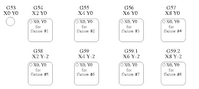
To use fixture offsets, the values of the desired home positions must be stored in the control, prior to running a program that uses them. Once there are values assigned, a call to G54, for instance, would add 2 to all X values in a program. A call to G58 would add 2 to X values and -2 to Y values in this example.
G53 is used to cancel out fixture offsets. So, calling G53 and then G0 X0 Y0 would send the machine back to the actual coordinates of X=0, Y=0.
G53 motion in machine coordinate system
G54 use preset work coordinate system 1
G55 use preset work coordinate system 2
G56 use preset work coordinate system 3
G57 use preset work coordinate system 4
G58 use preset work coordinate system 5
G59 use preset work coordinate system 6
G59.1 use preset work coordinate system 7
G59.2 use preset work coordinate system 8
G59.3 use preset work coordinate system 9
Canned Cycles/Drill Subroutines (G80-G89)
Distance ModesG90 absolute distance mode
G91 incremental distance mode
Feedrate and feed modesG93 inverse time feed mode
G94 feed per minute mode
Miscellaneous wordsM words are used to control many of the I/O functions of a machine. M words can start the spindle and turn on mist or flood coolant. M words also signal the end of a program or a stop withing a program. The complete list of M words available to the RS274NGC programmer is included below :
M Word List M0 program stop
M1 optional program stop
M2 program end
M3 turn spindle clockwise
M4 turn spindle counterclockwise
M5 stop spindle turning
M6 tool change
M7 mist coolant on M8 flood coolant on
M9 mist and flood coolant off
M26 enable automatic b-axis clamping
M27 disable automatic b-axis clamping
M30 program end, pallet shuttle, and reset
M48 enable speed and feed overrides
M49 disable speed and feed overrides
M60 pallet shuttle and program stop
Modal CodesMany G codes and M codes cause the machine to change from one mode to another, and the mode stays active until some other command changes it implicitly or explicitly . Such commands are called "modal".
Modal codes are like a light switch. Flip it on and the lamp stays lit until someone turns it off. For example, the coolant commands are modal. If coolant is turned on, it stays on until it is explicitly turned off. The G codes for motion are also modal. If a G1 (straight move) command is given on one line, it will be executed again on the next line unless a command is given specifying a different motion (or some other command which implicitly cancels G1 is given).
"Non-modal" codes effect only the lines on which they occur. For example, G4 (dwell) is non-modal.
Modal commands are arranged in sets called "modal groups". Only one member of a modal group may be in force at any given time. In general, a modal group contains commands for which it is logically impossible for two members to be in effect at the same time. Measurement in inches vs. measure in millimeters are modal. A machine tool may be in many modes at the same time, with one mode from each group being in effect.
G and M Code Modal Groupsgroup 1 = {G0, G1, G2, G3, G80, G81, G82, G83, G84, G85, G86, G87, G88, G89} - motion
group 2 = {G17, G18, G19} - plane selection
group 3 = {G90, G91} - distance mode
group 5 = {G93, G94} - spindle speed mode
group 6 = {G20, G21} - units
group 7 = {G40, G41, G42} - cutter diameter compensation
group 8 = {G43, G49} - tool length offset
group 10 = {G98, G99} - return mode in canned cycles
group12 = {G54, G55, G56, G57, G58, G59, G59.1, G59.2, G59.3} coordinate system selection
group 2 = {M26, M27} - axis clamping
group 4 = {M0, M1, M2, M30, M60} - stopping
group 6 = {M6} - tool change
group 7 = {M3, M4, M5} - spindle turning
group 8 = {M7, M8, M9} - coolant
group 9 = {M48, M49} - feed and speed override bypass
There is some question about the reasons why some codes are included in the modal group that surrounds them. But most of the modal groupings make sence in that only one state can be active at a time.


